
Abstract
Many GPS manufacturers tout binary protocols more dense than NMEA and baud rates higher than the NMEA-standard 4800 bps as ways to increase GPS performance. While working on gpsd, I became interested in evaluating these claims, which have some implications for the design of gpsd. Later, the average and peak latency became of interest for modeling the performance of GPS as a time service. This paper discusses the theory and the results of profiling the code, and reaches some conclusions about system tuning and latency control.
What Can We Measure and Improve?
The most important characteristic of a GPS, the positional accuracy of its fixes, is a function of the GPS system and receiver design; GPSD can do nothing to affect it. However, a GPS fix has a timestamp, and the transmission path from the GPS to a user application introduces some latency (that is, delay between the time of fix and when it is available to the user).
Latency could be significant source of position error for a GPS in motion. It may also be a significant issue if the GPS is being used as a high-precision time source.
This paper describes the results of two rounds of measurement using different tools. Both yielded interesting results, and can usefully be juxtaposed with one another.
The first round was performed in 2005 using a version of the code very near 2.13. This was before the JSON protocol change and before GPSD developed the capability to do automated cycle detection. Consequently the statistics extracted were primarily timings of individual packets coming over the wire from the GPS.
The second round was performed in 2011 using a version of the code between 3.1 and 3.2. At this time GPSD was being evaluated as a high-precision time source for use in measuring network latency and checking the performance of NTP. The profiling tools built into GPSD had been rebuilt with an emphasis on timing the entire GPS reporting cycle, rather than individual packets.
Both the 2005 and 2011 rounds used the same consumer-grade sensor attached via USB to a Linux machine via a USB link, reporting to gpsd which is polled via sockets by a profiling application. In all cases the GPS was stationary at approximately 40N 75W.
Per-sentence profiling
Modeling the reporting chain
Consider the whole transmission path of a TPV (position/velocity/time) report from a GPS to the user or user application. It has the following stages:
-
A TPV report is generated in the GPS
-
It is encoded (into NMEA or a vendor binary protocol) and buffered for transmission via serial link.
-
The encoding is transmitted via serial link to a buffer in gpsd.
-
The encoding is decoded and translated into a notification in GPSD’s protocol.
-
The GPSD-protocol notification is polled and read over a client socket.
-
The GPSD-protocol notification is decoded by libgps and unpacked into a session structure available to the user application.
It is also relevant that consumer-grade GPSes do not expect to be polled, but are designed to issue TPV reports on a fixed cycle time, which we’ll call C and which is usually 1 second. gpsd expects this. A few GPSes (notably SiRF-II-based ones) can be polled, and we might thus be able to pull TPV reports out of them at a higher rate. gpsd doesn’t do this; one question this investigation can address is whether there would be any point to that.
At various times GPS manufacturers have promoted proprietary binary protocols and transmission speeds higher than the NMEA-standard 4800bps as ways to improve GPS performance. Obviously these cannot affect positional accuracy; all they can change is the latency at stages 2, 3, and 4.
The implementation of gpsd affects how much latency is introduced at stage 4. The design of the gpsd protocol (in particular, the average and worst-case size and complexity of a position/velocity/time report) affects how much latency is introduced at stages 5 and 6.
At stages 5 and later, the client design and implementation matter a lot. In particular, it matters how frequently the client samples the TPV reports that gpsd makes available.
The list of stages above implies the following formula for expected latency L, and a set of tactics for reducing it:
L = C/2 + E1 + T1 + D1 + W + E2 + T2 + D2
where:
-
C/2 is the expected delay introduced by a cycle time of C (worst-case delay would just be C). We can decrease this by decreasing C, but consumer-grade GPSes don’t go below 1 second.
-
E1 is TPV encoding time within the GPS. We can’t affect this.
-
T1 is transmission time over the serial link. We can decrease this by raising the baud rate or increasing the information density of the encoding.
-
D1 is decode time required for gpsd to update its session structure. We can decrease this, if need be, by tuning the implementation or using faster hardware.
-
W is the wait until the application polls gpsd. This can only be reduced by designing the application to poll frequently.
-
E2 is TPV encoding time within the daemon. We can speed this up with faster hardware or a simpler GPSD format.
-
T2 is transmission time over the client socket. Faster hardware, a better TCP/IP stack or a denser encoding can decrease this.
-
D2 is decoding time required for the client library to update the session structure visible to the user application. A simpler GPSD format could decrease this
The total figure L is of interest, of course. The first question to ask is how it compares to C. But to know where tuning this system is worth the effort and where it isn’t, the relative magnitude of these six components is what is important. In particular, if C or E1 dominate, there is no point in trying to tune the system at all.
The rule on modern hardware is that computation is cheap, communication is expensive. By this rule, we expect E1, D1, E2, and D2 to be small relative to T1 and T2. We can’t predict W. Thus there is no knowing how the sum of the other terms will compare to C, but we know that E1 + T1 is the other statistic GPS vendors can easily measure. C < E1 + T1 would be a bad idea, and we can guess that competition among GPS vendors will probably tend to push C downwards to the point where it’s not much larger than E1 + T1.
C is known from manufacturer specifications. gpsd and its client libraries can be built with profiling code that measures all the other timing variables. The tool gpsprof1 collects this data and generates reports and plots from it. There are, however, some sources of error to be aware of:
-
Our way of measuring E1 and T1 is to collect a timestamp on the first character read of a new NMEA sentence, then on the terminating newline, and compare those to the GPS timestamp on the sentence. While this will measure E1+T1 accurately, it will underestimate the contribution of T1 to the whole because it doesn’t measure RS232 activity taking place before the first character becomes visible at the receive end.
-
Because we compare GPS sentence timestamps with local ones, inaccuracy in the computer’s clock fuzzes the measurements. The test machine updated time from NTP, so the expected inaccuracy from this source should be not more than about ten milliseconds.
-
The $ clause that the daemon uses to ship per-sentence profiling info to the client adds substantial bulk to the traffic. Thus, it will tend to inflate E2, T2, and D2 somewhat.
-
The client library used for profiling is written in Python, which will further inflate D2 relative to the C client library most applications are likely to use.
-
The system-call overhead of profiling (seven gettimeofday2 calls per sentence to collect timestamps, several other time-library calls per sentence to convert ISO8661 timestamps) will introduce a small amount of noise into the figures. These are cheap calls that don’t induce disk activity; thus, on modern hardware; we may expect the overhead per call to be at worst in the microsecond range. The entire per-sentence overhead system-call overhead should be on the order of ten microseconds.
Data and Analysis
I took measurements using a Haicom 204s USB GPS mouse. This device, using a SiRF-II GPS chipset and PL2303 USB-to-serial chipset, is very typical of 2005’s consumer-grade GPS hardware; the Haicom people themselves estimated to me in late 2004 that the SirF-II had about 80% and rising market share, and the specification sheets I find with Web searches back this up. Each profile run used 100 samples.
My host system for the measurements was an Opteron 3400 running an "everything" installation of Fedora Core 3. This was still a moderately fast machine in early 2005, but average processor utilization remained low throughout the tests.
The version of the GPSD software I used for the test was released as 2.13. It was configured with --enable-profiling. All graphs and figures were generated with gpsprof1, a tool built for this purpose and included in the distribution.
One of the effects of building with --enable-profiling is that a form of the B command that normally just reports the RS232 parameters can be used to set them (it ships a SiRF-II control string to the GPS and then changes the line settings).
Another effect is to enable a Z command to switch on profiling. When profiling is on, each time gpsd reports a fix with timestamp (e.g. on GPGGA, GPRMC and GPGLL sentences) it also reports timing information from five checkpoints inside the daemon. The client library adds two more checkpoints.
Our first graph is with profile reporting turned off, to give us a
handle on performance with the system disturbed as little as possible.
This was generated with gpsprof -t "Haicom 204s" -T png -f
uninstrumented -s 4800. We’ll compare it to later plots to see the
effect of profiling overhead.
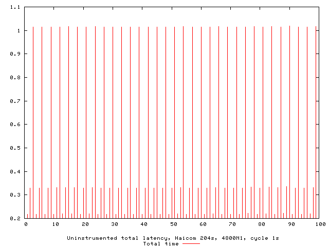
Uninstrumented total latency is simply the delta from the GPS timestamp associated with the packet to the arrival time of the end of the packet at the profiling client. The repeated stairstep effect is because all packets in a reporting cycle have the same timestamp; thus, the impulses cumulate time in the reporting cycle so far.
The first thing to notice here is that the fix latency can be just over
a second; you can see the exact figures in the raw
data. Where is the time going? Our next graph was generated with
gpsprof -T png -t
"Haicom 204s" -f raw -s 4800
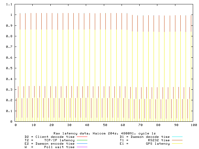
As in the previous graph, each group of three lines is a single GPS
reporting cycle. By comparing this graph to the previous one, it is
pretty clear that the profiling reports are not introducing any
measurable latency. But what is more interesting is to notice that D1
W + E2 + T2 + D2 vanishes — at this timescale, all we can see is E1
and T1.
The raw data bears this out. All times besides E1 and T1 are so small that they are comparable to the noise level of the measurements. This may be a bit surprising unless one knows that a W near 0 is expected in this setup; gpsprof sets watcher mode. Also, a modern zero-copy TCP/IP stack like Linux’s implements local sockets with very low overhead. It is also a little surprising that E1 is so large relative to E1+T1. Recall, however, that this may be measurement error.
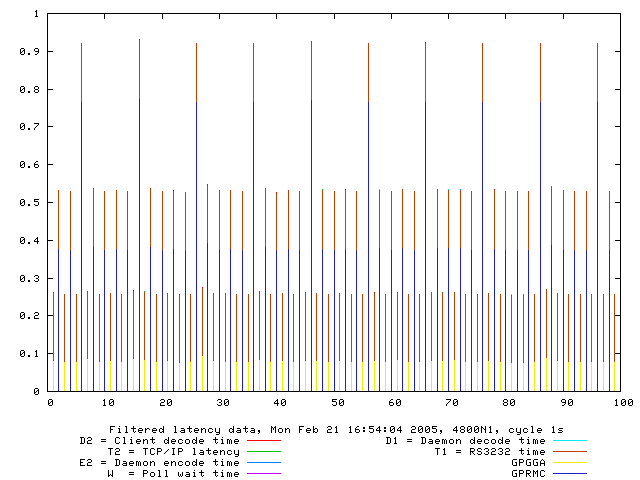
Our third graph (gpsprof -t "Haicom 204s" -T png -f split -s 4800
changes the presentation so we can see how latency varies with sentence
type.
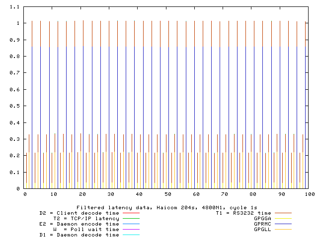
The reason for the comb pattern in the previous graphs is now apparent; latency is constant for any given sentence type. The obvious correlate would be sentence length — but looking at the raw data, we see that that is not the only factor. Consider this table:
| Sentence type | Typical length | Typical latency |
|---|---|---|
GPRMC |
70 |
1.01 |
GPGGA |
81 |
0.23 |
GPGLL |
49 |
0.31 |
For illustration, here are some sample NMEA sentences logged while I was conducting these tests:
$GPRMC,183424.834,A,4002.1033,N,07531.2003,W,0.00,0.00,170205,,*11
$GPGGA,183425.834,4002.1035,N,07531.2004,W,1,05,1.9,134.7,M,-33.8,M,0.0,0000*48
$GPGLL,4002.1035,N,07531.2004,W,183425.834,A*27
Though GPRMCs are shorter than GPGAs, they consistently have an associated latency four times as long. The graph tells us most of this is E1. There must be something the GPS is doing that is computationally very expensive when it generates GPRMCs. It may well be that it is actually doing that fix at that point in the send cycle and buffering the results for retransmission in GPGGA and GPGLL forms. Alternatively, perhaps the speed/track computation is expensive.
Now let’s look at how the picture changes when we double the baud rate.
gpsprof -t "Haicom 204s" -T png -s 9600 gives us this:
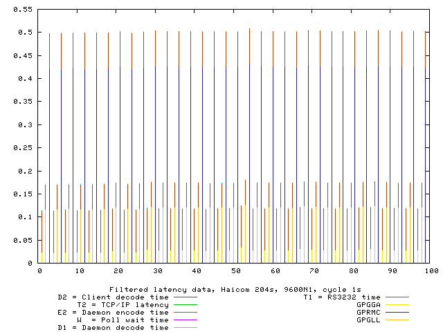
This graph looks almost identical to the previous one, except for vertical scale — latency has been cut neatly in half. Transmission times for GPRMC go from about 0.15sec to 0.075sec. Oddly, average E1 is also cut almost in half. I don’t know how to explain this, unless a lot of what looks like E1 is actually RS232 transmission time spent before the first character appears in the daemon’s receive buffers. You can also view the raw data.
For comparison, here’s the same plot made with a BU303b, a different USB GPS mouse using the same SiRF-II/PL2303 combination:
This, and the raw data, look very similar to the Haicom numbers. The main difference seems to be that the BU303b firmware doesn’t ship GPGLL by default.
Per-cycle profiling
Modeling the reporting chain
When the old GPSD protocol was replaced by an application of JSON and the daemon developed the capability to perform automatic detection of the beginning and end of GPS reporting cycles, it became possible to measure whole-cycle latency. Also, embedding timing statistics in the JSON digest of an entire cycle rather than as a $ sentence after each GPS packet significantly reduced the overhead of profiling in the report stream.
The model for these measurements is as follows:
-
A TPV report is generated in the GPS (at time 'T')
-
It is encoded into a burst of sentences in NMEA or a vendor binary protocol and buffered for transmission via serial link.
-
The encoding is transmitted via serial link to a buffer in gpsd, beginning at a time we shall call 'S'.
-
Because it consists of multiple packets, a period combining serial transmission time with gpsd processing (packet-sniffing and analysis) time will follow.
-
At the end of this interval (at a time we shall call 'E'), gpsd has seen the GPS data it needs and is ready to produce a report to ship to clients.
-
Meanwhile, the GPS may still be transmitting data that GPSD does not use. But when the transmission burst is done, there will be quiet time on the link (exception: as we noted in 2005, some devices' transmissions may slightly overflow the 1-second cycle time at 4800bps).
-
The JSON report is shipped, arriving at the client at a time we shall call 'R'.
We cannot know T directly. The GPS’s timestamp on the fix will tell us when it thinks T was, but because we don’t know how our local clock diverges from GPS’s atomic-clock timebase we don’t actually know what T was in system time (call that T'). If we trust NTP, we then believe that the skew between T and T' is no more than 10ms.
We catch time S by recording system time each time data becomes available from the device. If adjacent returns of select(2) are separated by more than 250msec, we have good reason to believe that the second one follows end-of-cycle quiet time. This guard interval is reliable at 9600bps and will only be more so at higher speeds.
We catch time E just before a JSON report is generated from the per-device session structures. This is the wnd of the analysis phase. If timing is enabled, extra members carrying S, E and the number of characters transmitted during the cycle © are included in the JSON.
We catch time R by noting when the JSON arrives at the client.
We know that the transmission-time portion of [S, E] can be approximated by the formula (C * 10) / B where B is the transmission rate in bits per second. (Each character costs 8 bits plus one parity bit plus one stop bit.)
Knowing this, we can subtract (C * 10) / B from (E-S) to approximate the internal processing time spent by gpsd. Due to other UART overheads, this formula will slightly underestimate transmission time and this overestimate processing time, but even a rough comparison of the two is interesting.
Data and Analysis
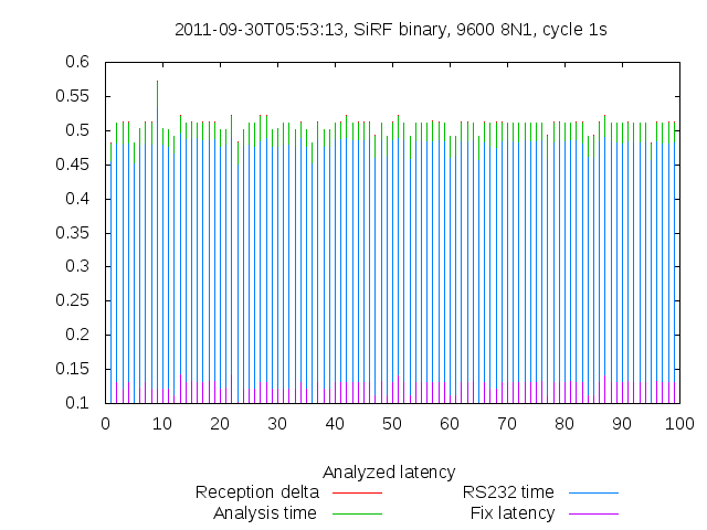
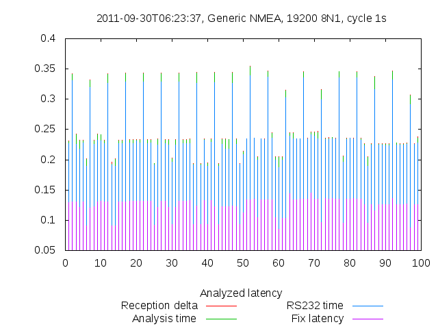
With the new profiling tools, one graph (made with gpsprof -f instrumented -n 100 -T png) tells the story. This is from the same Haicom 204s used in the 2005 tests. You can see the exact figures in the raw data.
Fix latency (S - T, the purple time segment in each sample) is consistently about 120msec. Some of this represents on-chip processing. Some may represent actual skew between NTP time and GPS time.
RS232 time (the blue segment) is the character transmission time estimate we computed. It seems relatively steady at around 125ms. This is probably a bit low, proportionately speaking.
The green segment is (E-S) with RS232 computed time subtracted. It approximates the time required by gpsd for itelf. It seems steady at around 15ms. This is probably a bit high, proportionately speaking.
The red dots that are just barely visible at the tops of some sample bars represent R-E, the client reception delta. Inspection of the raw data reveals that it is on the close order of 1ms.
Total fix latency is steady at about 310ms. Transmission time dominates.
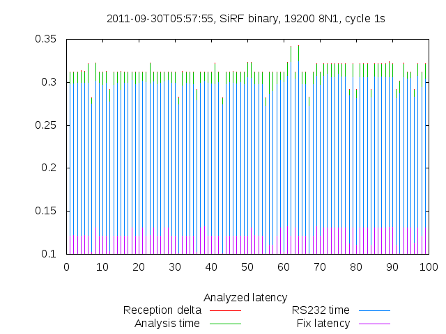
It is instructive to compare this with the graph (and the raw data) from the same device at 9600bps.
As we might expect, RS232 time changes drastically and the other components barely change at all. This gives us reason to be confident that computed RS232 time is in fact tracking actual transmission time pretty closely. It also confirms that the most effective way to decrease total fix latency is simply to bump up the transmission speed.
It is equally instructive to compare these graphs with graphs taken from the same GPS, at the same speed, running in NMEA rather than vendor binary mode. Consider, for example, these:
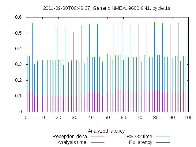
(Raw data is here.)
(Raw data is here.)
The comb-shaped pattern in these graphs reflect the additional transmission time for $GPGSV every 5 cycles. We can see clearly that the vendor binary protocol does not significantly cut either the latency or the total bandwidth required.
Conclusions
All these conclusions apply to the consumer-grade GPS hardware generally available back in 2005 and today in 2011, e.g. with a cycle time of one second. As it happens, 2005 was just after the point when consumer-grade GPS chips stabilized as a technology, and though unit prices have fallen they have changed relatively little in technology and performance over the intervening six years. The main improvement has been in sensitivity, improving operation with a poor skyview but not affecting the timing characteristics of the output.
For Application Programmers
For the best tradeoff between minimizing latency and use of application resources, an argument similar to Nyquist’s Theorem tells us to poll gpsd once every half-cycle — that is, on almost all GPSes at time of writing, twice a second.
With the SiRF chips still used in most consumer-grade GPSes at time of writing, 9600bps is the optimal line speed. 4800 is slightly too low, not guaranteeing updates within the 1-second cycle time. 9600bps yields updates in about 0.45sec, 19600bps in about 0.26sec. Higher speeds would probably not be worth the extra computation unless your sensor is in rapid motion. Even whole-cycle latency, most sensitive to transmission speed, is only cut by less than 200ms by going to 19200. Higher speed will exhibit diminishing returns.
Comparing the SiRF-II performance at 4800bps and 9600 shows a drop in E1+T1 that looks about linear, suggesting that for a cycle of n seconds, the optimal line speed would be about 9600/n. Since future GPS chips are likely to have faster processors and thus less latency, this may be considered an upper bound on useful line speed.
For Manufacturer Claims
Because 9600bps is readily available, the transmission- and decode-time advantages of binary protocols over NMEA are not significant within a 1-per-second update cycle. Because line speeds up to 38400 are readily available through standard UARTs, we may expect this to continue to be the case even with cycle times as low as 0.25sec.
More generally, binary protocols are largely pointless except as market-control devices for the manufacturers. The additional capabilities they support could be just as effectively supported through NMEA’s $P-prefix extension mechanism.
For GPSD as a Time Service
We have measured a typical intrisic time latency of about 70msec due to on-GPS processing and the USB polling interval. While this is noticeably higher than NTP’s expected accuracy of ±10msec, it should be adequate for most applications other than physics experiments.
For the Design of GPSD
In 2005, I wrote that gpsd does not introduce measurable latency into the path from GPS to application. I said that cycle times would have to decrease by two orders of magnitude for this to change.
In 2011, with better whole-cycle oriented profiling tools and a faster test machine, latency incurred by gpsd can be measured. It is less than 15ms sec on a 2.66 Intel Core Duo under normal load. How much less depends on how much the model computations underestimate RS232 transmission time for the GPS data.
Revision History
Revision |
Date |
Author |
Comments |
2.4 |
25 January 2020 |
gem |
Convert from DocBook to AsciiDoc |
2.3 |
25 November 2011 |
esr |
Typo fixes. |
2.2 |
30 September 2011 |
esr |
Fix errors in some whole-cycle visualizations. |
2.1 |
29 September 2011 |
esr |
Revisions as suggested by Hal Murray. |
2.0 |
23 September 2011 |
esr |
Update to include whole-cycle profiling. |
1.2 |
27 September 2009 |
esr |
Endnote about the big protocol change. |
1.1 |
4 January 2008 |
esr |
Typo fixes and clarifications for issues raised by Bruce Sutherland. |
1.0 |
21 February 2005 |
esr |
Initial draft. |
COPYING
This file is Copyright 2005 by the GPSD project This file is Copyright 2005 by Eric S. Raymond SPDX-License-Identifier: BSD-2-clause